Spotify Playlist Clustering: Exploratory Analysis
by Michael Marzec
I love the ease of adding a song to my Spotify ‘Liked Songs’, but I am admittedly too lazy to create and update playlists. This is fine until I want to shuffle my ‘Liked Songs’ and suddenly my playlist jumps from Prince to Leon Bridges to Spoon.
Spotify provides its users the option to filter their ‘Liked Songs’ by genre. While this offers a convenient solution, I feel that genre filters can lack a certain nuance. An album will be classified as a specific genre, but its tracklist can feature a variety of song types. For example, a “pop” album could feature a mixture of high-energy workout music, background melodies, and something to play during a family dinner.
Some artists are more inclined to create mixed-genre albums than others (e.g., James Blake, Beck, Kanye West). However, regardless of the artist or genre, I’d like to use this concept to create automated and customized playlists from my ‘Liked Songs’ Spotify library.
Data
Spotify provides a fantastic API to access their data and Spotipy makes it very easy to use. For this project, the API provides three key features:
- Download your ‘Liked Songs’.
- Extract key features for each song.
- Create and populate playlists.
The first and third points are fairly self-explanatory, but the ‘key features’ are a custom Spotify API output. These include characteristics like ‘danceability’, ‘energy’, and ‘tempo’ among others listed here. Thus, using these API functions, I can easily download a list of every liked song, about 12 descriptive variables for each song, and ultimately, group these songs into new playlists.
In my opinion, this solution’s most significant assumption is its reliance on Spotify’s pre-determined audio features. While they are convenient and easy to use, the solution is dependent on Spotify’s calculated audio features reliably encapsulating each song’s, for lack of a better word, vibe. Essentially, the audio features provide a great foundation for this project, but given the appropriate access, I would love to leverage audio files (e.g., .wav data) to analyze the raw audio data via a library such as ibrosa.
PCA
After extracting the descriptive variables, I standardized the data and applied principal component analysis (PCA), which among other benefits, reduces dimensionality and the risk of multicollinearity.
When using PCA, the end user needs to determine the number of ‘principal components’ to keep for any subsequent processing. There are a couple of typical options:
- Visualize the principal components using a scree plot and determine the appropriate number to keep via ‘elbow’ analysis.
- Determine the preferred variance to ‘capture’ via the principal components and let that determine the number to keep.
See the following for an example of a scree plot:
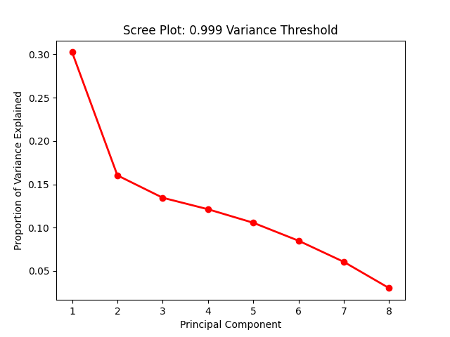
Elbow analysis suggests using an inflection point of significant change. At first glance, this suggests using two principal components. There is also precedence to using a ‘variance threshold’ approach. In later sections, I’ll discuss my evaluation methodology, which includes models that use two principal components versus a variance threshold.
Additionally, note that a customized environment often provides the opportunity to evaluate a scree plot and subsequently determine the optimal number of components. However, by choosing a variance threshold, the solution can be simplified and thus better prepared for scalable deployment.
Clustering
After selecting the principal components, this data can be fed to a clustering algorithm. The algorithm will separate each data point (i.e., song) into a different cluster. In this instance, each cluster will represent a playlist. I considered two approaches to determining the number of clusters:
- Non-Technical
- My ‘Liked Songs’ playlist consists of roughly 1500 songs. At 75 songs per playlist, I would specify 20 clusters. While there is nothing technical to this approach, 75 songs per playlist strikes me as a healthy balance between the number of playlists and songs per playlist.
- Technical
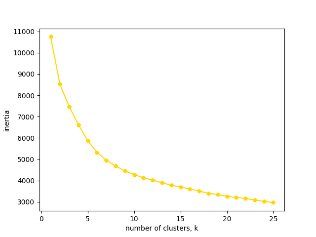
- The appropriate number of clusters can be analyzed via an inertia plot. Similar to PCA, it’s an inexact science that commonly uses the elbow method.
Using the following inertia plot, I selected 11 clusters (which frankly feels like an arbitrary decision) as my ‘technical’ approach for further evaluation:
Note that so far I’ve avoided mentioning which clustering algorithm is being implemented. To this point, I’ve used k-means clustering (via scikit-learn library). There are countless clustering algorithms, each of which uses another variation to achieve the same objective: sort each data point into groups with other similar data points.
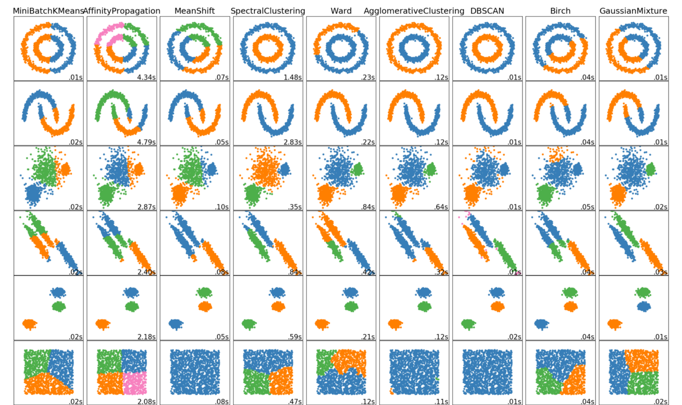
In the following evaluation section, I experiment with k-means, birch, dbscan, and gaussian clustering. The experiment results highlight some differences across each algorithm. However, the following graphic is a personal favorite which visualizes the results of a handful of clustering algorithms based on the data distribution:
Evaluation
Evaluating unsupervised exploratory analysis is inherently difficult. There are no “correct” answers to measure the results against (i.e., no Y / independent variable). I can evaluate the playlists using personal judgment, but any outcome assessment is subjective at best.
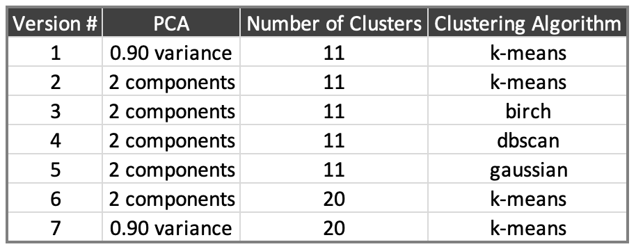
Altogether, I ran eight versions with the following parameters:
First, using clustering maps based on two principal components, the dbscan results stand out. This algorithm determines the number of clusters rather than allowing the user to decide. Per the following plot, there are only three clusters, and the patterns differ significantly from the other algorithms. For those reasons, I’ve ruled this out.
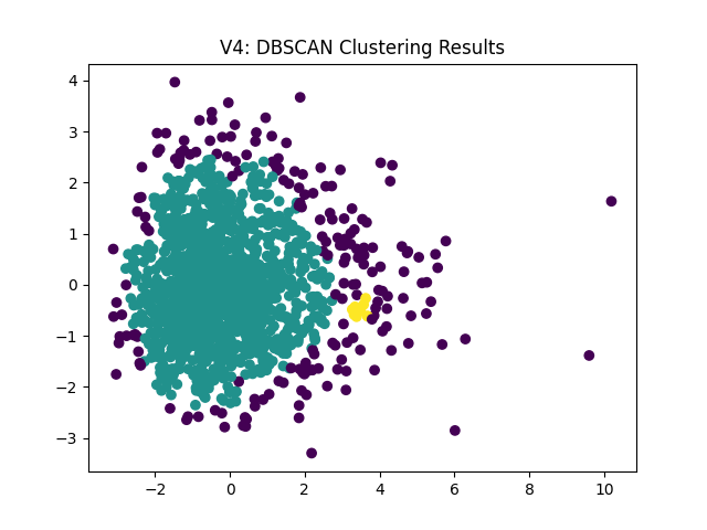
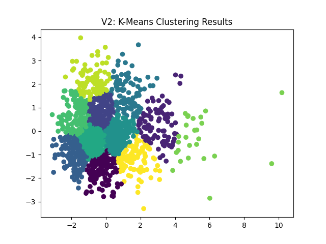
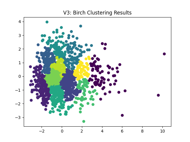
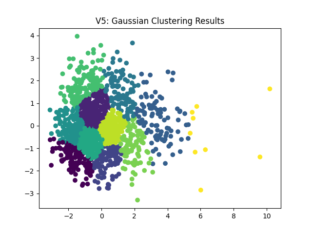
Next, we can see very similar cluster patterns from the remaining algorithms:
 |
 |
 |
Considering the similarity in the graphs, I’m going to move forward with the k-means algorithm (V2). The following shows 11 vs 20 playlists/clusters:
| |
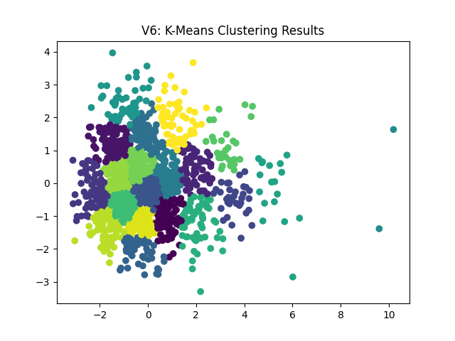 |
In all honesty, the cluster plots don’t leave me with a strong preference. There are a lot of similar groupings with slightly more granular breakdowns. As such, I’m going to move forward with 20 playlists (i.e., my non-technical approach) and, as mentioned, I’d prefer to use a variance threshold (rather than an ad-hoc principal component decision). This leaves me with V7 as my final model to create my customized Spotify playlists.
Conclusion and Future Efforts
Altogether, I am happy with my initial attempt at automated playlists. The playlists aren’t perfect (to be expected) but they seem to have some coherent similarities. A few additional concluding thoughts and ideas for future updates:
- I would like to add an output report (and/or title the playlists) based on the various audio features. For example, whichever playlist has the highest average ‘danceability’ could be named ‘autoPlaylist_dancetracks’.
- I want to develop end-to-end deployment for a casual end user. At a bare minimum, the parameters could be limited to the Spotify Client ID, Spotify Secret Code, Spotify username, and number of desired playlists. For advanced users, additional options could include the principal component threshold, preferred clustering algorithm, and whether to print the scree and inertia plots.
- Ideally, this could be completed via a simple hosted website or a local executable.
- I am still considering what a model rerun should look like… Should it retain the original model and predict (i.e., place) the newly liked songs into the existing playlists? Or should it delete all cluster-based playlists, retrain and recreate the playlists from scratch?
- In a functional application, this could be another advanced option for technical users with ‘delete and recreate’ as a default option.
- As mentioned, I would like to experiment with changing the input source to .wav/librosa data to remove dependency on Spotify’s audio features for comparison’s sake. Obtaining this data is probably unrealistic but still an interesting thought for future work.
- If you have any recommendations, questions, comments, etc. please feel free to reach out via email!